Graph

 A graph can be defined as group of vertices and edges that are used to connect these vertices. A graph can be seen as a cyclic tree, where the vertices (Nodes) maintain any complex relationship among them instead of having parent child relationship.

A graph G can be defined as an ordered set G(V, E) where V(G) represents the set of vertices and E(G) represents the set of edges which are used to connect these vertices.

A Graph G(V, E) with 5 vertices (A, B, C, D, E) and six edges ((A,B), (B,C), (C,E), (E,D), (D,B), (D,A)) is shown in the following figure.

Directed and Undirected Graph

A graph can be directed or undirected. However, in an undirected graph, edges are not associated with the directions with them. An undirected graph is shown in the above figure since its edges are not attached with any of the directions. If an edge exists between vertex A and B then the vertices can be traversed from B to A as well as A to B.

In a directed graph, edges form an ordered pair. Edges represent a specific path from some vertex A to another vertex B. Node A is called initial node while node B is called terminal node.

A directed graph is shown in the following figure

Graph Terminology

Path

A path can be defined as the sequence of nodes that are followed in order to reach some terminal node V from the initial node U.

Closed Path

A path will be called as closed path if the initial node is same as terminal node. A path will be closed path if V₀=V_N.

Simple Path

If all the nodes of the graph are distinct with an exception V₀=V_N, then such path P is called as closed simple path.

Cycle

A cycle can be defined as the path which has no repeated edges or vertices except the first and last vertices.

Connected Graph

A connected graph is the one in which some path exists between every two vertices (u, v) in V. There are no isolated nodes in connected graph.

Complete Graph

A complete graph is the one in which every node is connected with all other nodes. A complete graph contain n(n-1)/2 edges where n is the number of nodes in the graph.

Weighted Graph

In a weighted graph, each edge is assigned with some data such as length or weight. The weight of an edge e can be given as w(e) which must be a positive (+) value indicating the cost of traversing the edge.

Digraph

A digraph is a directed graph in which each edge of the graph is associated with some direction and the traversing can be done only in the specified direction.

Loop

An edge that is associated with the similar end points can be called as Loop.

Adjacent Nodes

If two nodes u and v are connected via an edge e, then the nodes u and v are called as neighbours or adjacent nodes.

Degree of the Node

A degree of a node is the number of edges that are connected with that node. A node with degree 0 is called as isolated node.

Graph representation

In this article, we will discuss the ways to represent the graph. By Graph representation, we simply mean the technique to be used to store some graph into the computer's memory.

A graph is a data structure that consist a sets of vertices (called nodes) and edges. There are two ways to store Graphs into the computer's memory:

• Sequential representation (or, Adjacency matrix representation)
• Linked list representation (or, Adjacency list representation)

In sequential representation, an adjacency matrix is used to store the graph. Whereas in linked list representation, there is a use of an adjacency list to store the graph.

Sequential representation

In sequential representation, there is a use of an adjacency matrix to represent the mapping between vertices and edges of the graph. We can use an adjacency matrix to represent the undirected graph, directed graph, weighted directed graph, and weighted undirected graph.

If adj[i][j] = w, it means that there is an edge exists from vertex i to vertex j with weight w.

An entry Aij in the adjacency matrix representation of an undirected graph G will be 1 if an edge exists between Vi and Vj. If an Undirected Graph G consists of n vertices, then the adjacency matrix for that graph is n x n, and the matrix A = [aij] can be defined as -

aij = 1 {if there is a path exists from Vi to Vj}

aij = 0 {Otherwise}

It means that, in an adjacency matrix, 0 represents that there is no association exists between the nodes, whereas 1 represents the existence of a path between two edges.

If there is no self-loop present in the graph, it means that the diagonal entries of the adjacency matrix will be 0.

In the above figure, an image shows the mapping among the vertices (A, B, C, D, E), and this mapping is represented by using the adjacency matrix.

There exist different adjacency matrices for the directed and undirected graph. In a directed graph, an entry Aij will be 1 only when there is an edge directed from Vi to Vj.

Adjacency matrix for a directed graph

In a directed graph, edges represent a specific path from one vertex to another vertex. Suppose a path exists from vertex A to another vertex B; it means that node A is the initial node, while node B is the terminal node.

Consider the below-directed graph and try to construct the adjacency matrix of it.

In the above graph, we can see there is no self-loop, so the diagonal entries of the adjacent matrix are 0.

Adjacency matrix for a weighted directed graph

It is similar to an adjacency matrix representation of a directed graph except that instead of using the '1' for the existence of a path, here we have to use the weight associated with the edge. The weights on the graph edges will be represented as the entries of the adjacency matrix. We can understand it with the help of an example. Consider the below graph and its adjacency matrix representation. In the representation, we can see that the weight associated with the edges is represented as the entries in the adjacency matrix.

Linked list representation

An adjacency list is used in the linked representation to store the Graph in the computer's memory. It is efficient in terms of storage as we only have to store the values for edges.

Let's see the adjacency list representation of an undirected graph.

In the above figure, we can see that there is a linked list or adjacency list for every node of the graph. From vertex A, there are paths to vertex B and vertex D. These nodes are linked to nodes A in the given adjacency list.

An adjacency list is maintained for each node present in the graph, which stores the node value and a pointer to the next adjacent node to the respective node. If all the adjacent nodes are traversed, then store the NULL in the pointer field of the last node of the list.

The sum of the lengths of adjacency lists is equal to twice the number of edges present in an undirected graph.

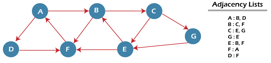
Now, consider the directed graph, and let's see the adjacency list representation of that grap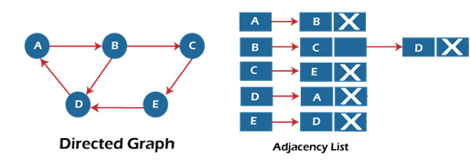

For a directed graph, the sum of the lengths of adjacency lists is equal to the number of edges present in the graph.

Now, consider the weighted directed graph, and let's see the adjacency list representation of that graph.

In the case of a weighted directed graph, each node contains an extra field that is called the weight of the node.

Breadth-first search 

Breadth-first search is a graph traversal algorithm that starts traversing the graph from the root node and explores all the neighboring nodes. Then, it selects the nearest node and explores all the unexplored nodes. While using BFS for traversal, any node in the graph can be considered as the root node.

There are many ways to traverse the graph, but among them, BFS is the most commonly used approach. It is a recursive algorithm to search all the vertices of a tree or graph data structure. BFS puts every vertex of the graph into two categories - visited and non-visited. It selects a single node in a graph and, after that, visits all the nodes adjacent to the selected node.

Example of BFS algorithm

Now, let's understand the working of BFS algorithm by using an example. In the example given below, there is a directed graph having 7 vertices.

In the above graph, minimum path 'P' can be found by using the BFS that will start from Node A and end at Node E. The algorithm uses two queues, namely QUEUE1 and QUEUE2. QUEUE1 holds all the nodes that are to be processed, while QUEUE2 holds all the nodes that are processed and deleted from QUEUE1.

DFS (Depth First Search) algorithm

It is a recursive algorithm to search all the vertices of a tree data structure or a graph. The depth-first search (DFS) algorithm starts with the initial node of graph G and goes deeper until we find the goal node or the node with no children.

Because of the recursive nature, stack data structure can be used to implement the DFS algorithm. The process of implementing the DFS is similar to the BFS algorithm.

The step by step process to implement the DFS traversal is given as follows -

1. First, create a stack with the total number of vertices in the graph.
2. Now, choose any vertex as the starting point of traversal, and push that vertex into the stack.
3. After that, push a non-visited vertex (adjacent to the vertex on the top of the stack) to the top of the stack.
4. Now, repeat steps 3 and 4 until no vertices are left to visit from the vertex on the stack's top.
5. If no vertex is left, go back and pop a vertex from the stack.
6. Repeat steps 2, 3, and 4 until the stack is empty.

Example of DFS algorithm

Now, let's understand the working of the DFS algorithm by using an example. In the example given below, there is a directed graph having 7 vertices.

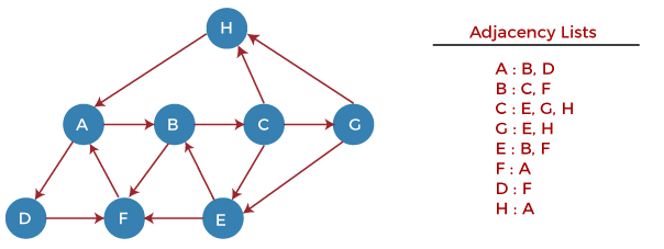
Now, let's start examining the graph starting from Node H